
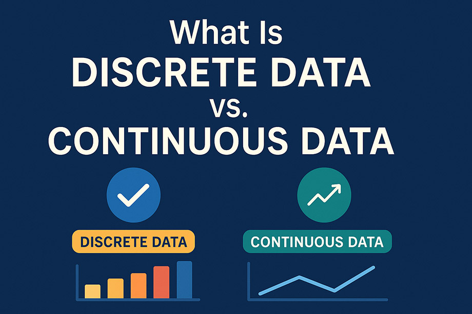
Discrete vs Continuous Data: Complete Guide with Examples & Applications
Understanding the fundamental difference between discrete and continuous data is crucial for accurate data analysis and business decision-making. Here’s everything you need to know.
In today’s data-driven world, we generate approximately 2.5 quintillion bytes of data every single day. From sending text messages to streaming videos, every digital interaction contributes to this massive data pool. However, not all data is created equal, and understanding the different types of data is crucial for effective analysis and decision-making.
Two fundamental categories of quantitative data that every analyst, researcher, and business professional should understand are discrete data and continuous data. While both represent numerical information, they have distinct characteristics that affect how we collect, analyze, visualize, and interpret them.
This comprehensive guide will explore the key differences between discrete and continuous data, provide practical examples, and explain when and how to use each type effectively.
Understanding Quantitative Data
Before diving into the specifics of discrete and continuous data, it’s essential to understand their place in the broader data classification system.
The Data Hierarchy
All Data ├── Qualitative (Categorical) Data │ ├── Nominal (e.g., colors, names) │ └── Ordinal (e.g., ratings, rankings) └── Quantitative (Numerical) Data ├── Discrete Data (countable) └── Continuous Data (measurable)
Quantitative data, also known as numerical data, represents information in the form of numbers that can be measured, counted, or calculated. This type of data allows for mathematical operations and statistical analysis, making it invaluable for data-driven decision making.
The two main types of quantitative data are:
- Discrete Data: Values that can be counted and have clear gaps between them
- Continuous Data: Values that can be measured and exist on a continuum
What is Discrete Data?
Definition and Characteristics
Discrete data refers to numerical information that can only take specific, distinct values. These values are typically whole numbers or integers that represent countable items or events.
Key Characteristics:
- Countable: You can count discrete data points
- Finite values: Limited number of possible values within any given range
- Clear gaps: Distinct spaces between possible values
- Indivisible: Cannot be meaningfully broken down into smaller parts
- Often integers: Usually whole numbers, though not exclusively
The “Number of” Test
A simple way to identify discrete data is to see if you can prefix it with “the number of”:
- The number of customers in your store
- The number of employees in your department
- The number of clicks on your website
- The number of products sold today
Common Examples of Discrete Data
Business and Commerce:
- Number of sales transactions
- Customer satisfaction ratings (1-10 scale)
- Number of website visitors
- Inventory count
- Number of support tickets
Demographics and Surveys:
- Number of family members
- Number of pets owned
- Age in years (whole numbers)
- Number of cars in a household
- Years of experience
Technology and Digital:
- Number of downloads
- Social media likes and shares
- Number of software bugs
- Server response codes
- Number of active users
Academic and Research:
- Number of students in a class
- Test scores (when using whole numbers)
- Number of research participants
- Published papers count
- Citation numbers
Discrete Data Subtypes
Binary Data: Only two possible values (0/1, Yes/No, True/False)
- Example: Customer subscription status (active/inactive)
Count Data: Non-negative integers representing frequencies
- Example: Number of product returns per month
Ordinal Discrete Data: Discrete values with meaningful order
- Example: Star ratings (1, 2, 3, 4, 5 stars)
What is Continuous Data?
Definition and Characteristics
Continuous data represents numerical information that can take any value within a given range or interval. This data is measured rather than counted and can theoretically have infinite precision.
Key Characteristics:
- Measurable: You measure continuous data using instruments
- Infinite possibilities: Unlimited values within any range
- No gaps: Values exist on a continuum
- Divisible: Can be broken down into smaller, meaningful parts
- Often includes decimals: Frequently expressed with decimal places
The Measurement Test
Continuous data typically involves measurements of:
- Time: Duration, intervals, timestamps
- Physical properties: Weight, height, temperature, distance
- Financial values: Prices, costs, revenue (when precise)
- Performance metrics: Speed, efficiency, ratios
Common Examples of Continuous Data
Physical Measurements:
- Height and weight of individuals
- Temperature readings
- Distance traveled
- Speed and velocity
- Blood pressure readings
Time-Related Data:
- Duration of phone calls
- Time to complete tasks
- Age (when measured precisely, including months/days)
- Response times
- Processing times
Financial and Business Metrics:
- Revenue and profit margins
- Stock prices
- Exchange rates
- Interest rates
- Customer lifetime value
Scientific and Technical:
- Chemical concentrations
- Electrical measurements (voltage, current)
- Frequency and wavelength
- Pressure readings
- pH levels
Continuous Data Subtypes
Interval Data: Equal intervals but no true zero point
- Example: Temperature in Celsius or Fahrenheit
Ratio Data: Equal intervals with a meaningful zero point
- Example: Weight, height, income
Key Differences Between Discrete and Continuous Data
Comprehensive Comparison Table
| Aspect | Discrete Data | Continuous Data |
|---|---|---|
| Nature | Countable, distinct values | Measurable, infinite possibilities |
| Values | Specific, separated points | Any value within a range |
| Gaps | Clear spaces between values | No gaps, continuous spectrum |
| Precision | Fixed precision | Theoretically infinite precision |
| Mathematical Operations | Limited (counting, frequency) | Full range (mean, standard deviation) |
| Visualization | Bar charts, pie charts | Histograms, line graphs |
| Statistical Tests | Chi-square, binomial tests | T-tests, ANOVA, regression |
| Examples | Number of customers | Customer satisfaction scores |
| Collection Method | Counting | Measuring with instruments |
Fundamental Differences Explained
1. Nature of Values
Discrete Data:
- Can only take specific, distinct values
- Example: You can have 5 or 6 customers, but not 5.3 customers
Continuous Data:
- Can take any value within a range
- Example: Temperature can be 23.7°C, 23.75°C, or 23.751°C
2. Precision and Measurement
Discrete Data:
- Precision is inherently limited by the nature of what’s being counted
- Values are exact and cannot be subdivided meaningfully
Continuous Data:
- Precision is limited only by the measuring instrument
- Can theoretically be measured to infinite decimal places
3. Gaps Between Values
Discrete Data:
- Clear gaps exist between possible values
- No meaningful values exist between consecutive integers
Continuous Data:
- No gaps between values
- Infinite possible values exist between any two points
4. Analysis Methods
Discrete Data:
- Focus on frequencies, counts, and proportions
- Mode is the most appropriate measure of central tendency
- Limited by the nature of whole numbers
Continuous Data:
- Can calculate mean, median, mode, and various statistical measures
- Allows for more sophisticated statistical analyses
- Can show trends and patterns over time
Examples in Real-World Applications
Healthcare Industry
Discrete Data Examples:
- Number of patients treated per day
- Number of hospital beds occupied
- Count of medical procedures performed
- Number of staff members on duty
- Patient satisfaction ratings (1-10 scale)
Continuous Data Examples:
- Patient vital signs (blood pressure, heart rate)
- Body measurements (height, weight, BMI)
- Medication dosages
- Treatment duration times
- Laboratory test results (blood glucose levels)
Mixed Application: A hospital might track both the number of emergency room visits (discrete) and the average wait time (continuous) to improve patient care.
E-commerce and Retail
Discrete Data Examples:
- Number of products in inventory
- Customer order quantities
- Number of website visitors
- Product review counts
- Number of returns or exchanges
Continuous Data Examples:
- Product prices and costs
- Shipping weights
- Customer lifetime value
- Website loading times
- Conversion rates (as percentages)
Business Impact: An online retailer might analyze the number of abandoned shopping carts (discrete) alongside the average time spent on product pages (continuous) to optimize the purchase process.
Manufacturing and Operations
Discrete Data Examples:
- Number of units produced
- Count of defective products
- Number of machine breakdowns
- Workforce headcount
- Number of safety incidents
Continuous Data Examples:
- Production line speed
- Material costs per unit
- Energy consumption
- Temperature and pressure readings
- Equipment efficiency ratios
Quality Control: Manufacturers often combine both data types, tracking the number of quality control inspections (discrete) and the dimensional measurements of products (continuous).
Digital Marketing and Analytics
Discrete Data Examples:
- Number of social media followers
- Email open counts
- Number of form submissions
- Click-through counts
- Number of active campaigns
Continuous Data Examples:
- Campaign ROI percentages
- Customer acquisition costs
- Time spent on website pages
- Bounce rates
- Conversion rates
Optimization Strategy: Digital marketers might analyze the number of email campaigns sent (discrete) against the average engagement time (continuous) to refine their strategies.
Data Visualization Methods
Discrete Data Visualization
Bar Charts
Best for: Comparing categories or showing frequencies Example: Number of sales by product category
Product A  ████████████████████ 45
Product B  ███████████████      35
Product C  ██████████           24
Product D  ████████             18
When to use:
- Comparing different categories
- Showing exact counts or frequencies
- Displaying survey results with distinct options
Pie Charts
Best for: Showing proportions of a whole Example: Distribution of customer types
When to use:
- Data represents parts of a whole (totaling 100%)
- Limited number of categories (5-7 maximum)
- Emphasizing relative proportions
Dot Plots
Best for: Simple frequency displays Example: Number of daily website visitors
When to use:
- Small datasets
- Emphasizing individual data points
- Comparing frequencies across categories
Stem-and-Leaf Plots
Best for: Showing distribution while preserving original values Example: Test scores (whole numbers)
When to use:
- Small to medium datasets
- Need to see both distribution and actual values
- Educational or exploratory analysis
Continuous Data Visualization
Histograms
Best for: Showing distribution patterns Example: Distribution of customer ages
When to use:
- Large datasets
- Understanding data distribution (normal, skewed, bimodal)
- Identifying outliers and patterns
Line Graphs
Best for: Showing trends over time Example: Revenue growth over months
When to use:
- Time series data
- Showing trends and patterns
- Comparing multiple continuous variables
Scatter Plots
Best for: Showing relationships between two continuous variables Example: Height vs. weight correlation
When to use:
- Exploring correlations
- Identifying outliers
- Regression analysis
Box Plots
Best for: Showing distribution summary statistics Example: Salary ranges by department
When to use:
- Comparing distributions across groups
- Identifying outliers
- Showing quartiles and median
Choosing the Right Visualization
| Data Type | Primary Charts | Secondary Options | Avoid |
|---|---|---|---|
| Discrete | Bar charts, Pie charts | Dot plots, Stem-and-leaf | Line graphs, Histograms |
| Continuous | Histograms, Line graphs | Box plots, Scatter plots | Pie charts (usually) |
| Mixed | Side-by-side comparisons | Combination charts | Single chart for both |
Statistical Analysis Approaches
Discrete Data Analysis
Descriptive Statistics
Frequency Analysis:
- Count how often each value appears
- Calculate percentages and proportions
- Identify mode (most frequent value)
Central Tendency:
- Mode: Most appropriate for discrete data
- Median: Useful for ordinal discrete data
- Mean: Can be calculated but may not be meaningful (e.g., average number of children per family = 2.3)
Common Statistical Tests
Chi-Square Tests:
- Test relationships between categorical variables
- Goodness of fit testing
- Independence testing
Binomial Tests:
- Analyze binary outcomes
- Proportion testing
- Success/failure scenarios
Poisson Analysis:
- Analyze count data
- Rate of occurrence over time
- Rare event modeling
Example Analysis
Customer Support Tickets per Day (Discrete Data):
Day 1: 15 tickets
Day 2: 23 tickets
Day 3: 18 tickets
Day 4: 31 tickets
Day 5: 12 tickets

Analysis:
- Total tickets: 99
- Average: 19.8 tickets/day
- Mode: No repeated values
- Range: 12-31 tickets
Continuous Data Analysis
Descriptive Statistics
Measures of Central Tendency:
- Mean: Average value (most common)
- Median: Middle value (robust to outliers)
- Mode: Peak of distribution
Measures of Variability:
- Standard Deviation: Spread around the mean
- Variance: Squared deviations
- Range: Difference between max and min
- Interquartile Range: Middle 50% spread
Advanced Analysis
Distribution Analysis:
- Normal distribution testing
- Skewness and kurtosis
- Outlier identification
Hypothesis Testing:
- T-tests for comparing means
- ANOVA for multiple groups
- Regression analysis for relationships
Example Analysis
Customer Response Times (Continuous Data):
Sample: 2.3, 1.8, 3.1, 2.7, 1.9, 2.4, 3.3, 2.1, 2.8, 2.5 seconds

Analysis:
- Mean: 2.49 seconds
- Median: 2.45 seconds
- Standard Deviation: 0.52 seconds
- Range: 1.8 - 3.3 seconds
- 95% of responses within: 1.45 - 3.53 seconds
Mixed Data Analysis
When working with both discrete and continuous data:
Correlation Analysis:
- Examine relationships between different data types
- Example: Number of employees (discrete) vs. revenue (continuous)
Segmentation:
- Group continuous data into discrete categories
- Example: Age ranges (18-25, 26-35, etc.)
Regression Modeling:
- Use discrete variables as predictors for continuous outcomes
- Include categorical variables in continuous models
Measurement Scales and Tools
Discrete Data Measurement
Nominal Scale
Characteristics:
- Categories with no inherent order
- Numbers used as labels only
- Cannot perform arithmetic operations
Examples:
- Customer ID numbers
- Product categories (1=Electronics, 2=Clothing, 3=Books)
- Gender coding (1=Male, 2=Female)
Analysis Methods:
- Frequency counts
- Mode calculation
- Chi-square tests
Ordinal Scale
Characteristics:
- Categories with meaningful order
- Differences between values not necessarily equal
- Can rank but not measure distance
Examples:
- Satisfaction ratings (1=Poor, 2=Fair, 3=Good, 4=Excellent)
- Education levels (1=High School, 2=Bachelor’s, 3=Master’s, 4=PhD)
- Performance rankings
Analysis Methods:
- Median calculation
- Percentile analysis
- Non-parametric tests
Continuous Data Measurement
Interval Scale
Characteristics:
- Equal intervals between values
- No true zero point
- Can measure differences but not ratios
Examples:
- Temperature in Celsius or Fahrenheit
- Calendar years
- IQ scores
Analysis Methods:
- Mean and standard deviation
- Correlation analysis
- T-tests and ANOVA
Ratio Scale
Characteristics:
- Equal intervals with true zero point
- Can perform all mathematical operations
- Most flexible for analysis
Examples:
- Height, weight, income
- Time durations
- Counts and frequencies
Analysis Methods:
- All statistical measures applicable
- Ratio comparisons meaningful
- Full range of parametric tests
Data Collection Tools
For Discrete Data
Counting Methods:
- Manual tallying
- Automated counters (web analytics)
- Sensor-based counting
- Survey responses with fixed options
Digital Tools:
- Google Analytics (page views, sessions)
- CRM systems (customer counts)
- Inventory management systems
- Social media analytics
For Continuous Data
Measurement Instruments:
- Digital scales and rulers
- Thermometers and gauges
- Timers and stopwatches
- Sensors and monitors
Software Tools:
- Data loggers
- IoT devices
- Financial systems (precise calculations)
- Scientific instruments
Common Misconceptions
Misconception 1: “Discrete Data Must Be Whole Numbers”
Reality: While discrete data is often represented by integers, it’s not limited to whole numbers.
Examples:
- Shoe sizes: 7, 7.5, 8, 8.5 (discrete because only specific sizes exist)
- Star ratings: 1, 1.5, 2, 2.5, 3, 3.5, 4, 4.5, 5 (discrete values on a rating scale)
- Test scores: Could be 85, 87.5, 90 (discrete if only certain scores are possible)
Key Point: The defining characteristic is the presence of gaps between possible values, not whether they’re whole numbers.
Misconception 2: “Money Is Always Continuous Data”
Reality: Money can be either discrete or continuous depending on context and precision.
Discrete Examples:
- Coin counts (1, 2, 3 coins)
- Dollar amounts when precision matters ($1, $2, $3, not $2.50)
- Pricing tiers ($9.99, $19.99, $29.99)
Continuous Examples:
- Precise financial calculations ($234.567)
- Exchange rates (1.23456 EUR/USD)
- Investment returns (12.34567%)
Misconception 3: “Age Is Always Discrete”
Reality: Age representation depends on precision and context.
Discrete Examples:
- Age in completed years (18, 19, 20 years old)
- Age groups (18-25, 26-35, 36-45)
Continuous Examples:
- Precise age (18.5 years, 18 years 6 months 2 days)
- Age for scientific calculations
- Life insurance actuarial calculations
Misconception 4: “Continuous Data Is Always More Valuable”
Reality: Both data types have unique strengths and appropriate use cases.
Discrete Data Advantages:
- Easier to understand and communicate
- Clear, unambiguous values
- Suitable for counting and categorization
- Less prone to measurement errors
Continuous Data Advantages:
- More statistical analysis options
- Better for modeling and prediction
- Can capture subtle variations
- Suitable for trend analysis
Misconception 5: “You Can Always Convert Between Types”
Reality: Conversion often results in information loss.
Discrete to Continuous Issues:
- Adding artificial precision where none exists
- Creating false continuity
- May not reflect true underlying processes
Continuous to Discrete Issues:
- Loss of precision and information
- Arbitrary boundary decisions
- Reduced analytical options
Practical Applications in Business
Marketing and Customer Analytics
Customer Segmentation
Discrete Approach:
Customer Types:
- New Customers: 245
- Returning Customers: 1,203
- VIP Customers: 67
- Churned Customers: 189
Continuous Approach:
Customer Metrics:
- Average Purchase Value: $67.23
- Customer Lifetime Value: $1,234.56
- Time Since Last Purchase: 23.5 days
- Engagement Score: 78.9%
Combined Analysis: Link discrete customer categories with continuous behavioral metrics to create comprehensive customer profiles.
Campaign Performance
Discrete Metrics:
- Number of campaigns launched
- Email open counts
- Click-through counts
- Conversion counts
Continuous Metrics:
- Campaign ROI percentages
- Cost per acquisition
- Customer lifetime value impact
- Time spent engaging with content
Operations and Supply Chain
Inventory Management
Discrete Data Applications:
- Stock levels and reorder points
- Number of suppliers
- Delivery frequency
- Product variety counts
Continuous Data Applications:
- Storage costs per unit
- Lead times and delivery times
- Quality scores and ratings
- Demand forecasting models
Quality Control
Discrete Monitoring:
Daily Quality Metrics:
- Units inspected: 500
- Defects found: 12
- Batches rejected: 3
- Inspector assignments: 5
Continuous Monitoring:
Quality Measurements:
- Average defect rate: 2.4%
- Process capability index: 1.33
- Temperature variance: ±2.1°C
- Dimension tolerances: ±0.05mm
Financial Analysis
Revenue Analysis
Discrete Perspective:
- Number of transactions
- Customer count by segment
- Product sales quantities
- Sales team performance rankings
Continuous Perspective:
- Revenue per transaction
- Profit margins
- Customer acquisition costs
- Growth rates and trends
Budget Planning
Discrete Budgeting:
Resource Allocation:
- Number of employees: 150
- Office locations: 5
- Software licenses: 200
- Equipment units: 75
Continuous Budgeting:
Financial Metrics:
- Personnel costs: $2.3M annually
- Office lease rates: $45/sq ft
- Software costs: $125/user/month
- Equipment depreciation: 20% annually
Human Resources
Workforce Analytics
Discrete HR Metrics:
- Employee headcount
- New hires per month
- Training sessions completed
- Performance rating categories
Continuous HR Metrics:
- Employee satisfaction scores
- Turnover rates
- Average tenure
- Productivity indices
Performance Management
Discrete Elements:
- Performance review cycles
- Goal achievement counts
- Training program completions
- Promotion eligibility categories
Continuous Elements:
- Performance scores (0-100)
- 360-degree feedback ratings
- Skill assessment scores
- Compensation adjustments
Best Practices for Data Collection
Planning Your Data Collection Strategy
1. Define Your Research Questions
For Discrete Data:
- How many [items/events/people] are there?
- What are the frequencies of different categories?
- Which category is most/least common?
For Continuous Data:
- What is the average/typical value?
- How much variation exists?
- What trends are present over time?
2. Choose Appropriate Data Types
Consider These Factors:
- Purpose: What will you do with the data?
- Precision: How exact do measurements need to be?
- Resources: What tools and time are available?
- Analysis: What statistical methods will you use?
Data Collection Methods
Discrete Data Collection
Counting Strategies:
- Manual counting: For small, controllable datasets
- Automated counting: Using sensors, software, or digital tools
- Sampling: When complete counts are impractical
- Categorization: Ensuring clear, mutually exclusive categories
Quality Assurance:
- Define clear counting rules
- Train data collectors consistently
- Implement validation checks
- Regular accuracy audits
Continuous Data Collection
Measurement Strategies:
- Instrument calibration: Ensure measurement accuracy
- Multiple measurements: Reduce random errors
- Standardized procedures: Consistent measurement methods
- Environmental controls: Minimize external influences
Precision Considerations:
- Significant figures: Match precision to purpose
- Measurement error: Understand and document limitations
- Sampling frequency: Balance accuracy with resources
- Data storage: Maintain precision through processing
Data Quality Management
Common Quality Issues
Discrete Data Problems:
- Miscounting: Human error in tallying
- Double counting: Including items multiple times
- Missing categories: Incomplete classification systems
- Inconsistent definitions: Changing criteria over time
Continuous Data Problems:
- Measurement drift: Instrument accuracy changes
- Rounding errors: Inappropriate precision loss
- Outliers: Extreme values affecting analysis
- Missing values: Incomplete measurements
Quality Improvement Strategies
Validation Techniques:
- Range checks: Ensure values fall within expected limits
- Consistency checks: Verify logical relationships
- Cross-validation: Compare with independent sources
- Statistical outlier detection: Identify unusual values
Documentation Standards:
- Data dictionaries: Define all variables clearly
- Collection procedures: Document methodology
- Change logs: Track modifications over time
- Quality metrics: Monitor data quality indicators
Technology Integration
Digital Collection Tools
For Discrete Data:
- Web analytics: Automated visitor and behavior counting
- CRM systems: Customer and interaction tracking
- IoT sensors: Event and occurrence counting
- Survey platforms: Response collection and categorization
For Continuous Data:
- Data loggers: Automated environmental monitoring
- Financial systems: Precise transaction recording
- Performance monitoring: System and process metrics
- Scientific instruments: Laboratory and field measurements
Data Integration Challenges
Common Issues:
- Format inconsistencies: Different systems use different formats
- Timing misalignment: Data collected at different intervals
- Scale differences: Various units and precision levels
- Quality variations: Different accuracy and completeness levels
Solution Strategies:
- Standardization protocols: Consistent formats and units
- Integration platforms: Centralized data management
- Quality scoring: Rate data source reliability
- Automated validation: Real-time quality checking
Conclusion: Making Data-Driven Decisions
Understanding the distinction between discrete and continuous data is fundamental to effective data analysis and business intelligence. This knowledge impacts every stage of the data lifecycle, from collection and storage to analysis and visualization.
Key Takeaways
For Discrete Data:
- Focus on counting, frequencies, and categorical analysis
- Use appropriate visualization methods (bar charts, pie charts)
- Apply suitable statistical tests (chi-square, binomial)
- Recognize limitations in precision and mathematical operations
For Continuous Data:
- Emphasize measurement, trends, and statistical modeling
- Use appropriate visualization methods (histograms, line graphs)
- Apply comprehensive statistical analyses (regression, ANOVA)
- Take advantage of full mathematical operation capabilities
Strategic Implications
Business Intelligence:
- Combine both data types for comprehensive insights
- Choose appropriate metrics for different business questions
- Align data collection methods with analytical goals
- Invest in proper tools and training for each data type
Decision Making:
- Use discrete data for operational decisions (staffing, inventory)
- Use continuous data for strategic decisions (pricing, forecasting)
- Understand the limitations and strengths of each approach
- Validate findings using multiple data perspectives
Future Considerations
As businesses become increasingly data-driven, the ability to work effectively with both discrete and continuous data becomes more critical. Advanced analytics, machine learning, and artificial intelligence often require sophisticated understanding of data types to produce accurate and actionable insights.
Whether you’re analyzing customer behavior, optimizing operations, or planning strategic initiatives, recognizing when to count versus when to measure—and how to analyze each appropriately—will significantly improve your ability to extract value from data and make informed decisions.
Remember: the goal isn’t to choose between discrete and continuous data, but to understand when and how to use each type effectively to answer your specific business questions and drive meaningful outcomes.
Ready to Apply These Concepts?
Start by examining your current data collection practices. Identify which metrics are discrete versus continuous, evaluate whether you’re using appropriate analysis methods, and consider how better understanding these distinctions could improve your decision-making processes.
The journey to data mastery begins with understanding these fundamental concepts and applying them consistently in your work.